What Are Sklearn Regression Models?
Regression models are an essential component of machine learning, enabling computers to make predictions and understand patterns in data without explicit programming. Sklearn, a powerful machine learning library, offers a range of regression models to facilitate this process.
Before delving into the specific regression methods in Sklearn, let’s briefly explore the three types of machine learning models that can be implemented using Sklearn Regression Models:
- reinforced learning,
- unsupervised learning
- supervised learning
These models allow computers to learn from data, make decisions, and perform tasks autonomously. Now, let’s take a closer look at some of the most popular regression methods available in Sklearn for implementing these models.
Linear Regression
Linear regression is a statistical modeling technique that aims to establish a linear relationship between a dependent variable and one or more independent variables. It assumes that there is a linear association between the independent variables and the dependent variable, and that the residuals (the differences between the actual and predicted values) are normally distributed.
Working principle of linear regression
The working principle of linear regression involves fitting a line to the data points that minimizes the sum of squared residuals. This line represents the best linear approximation of the relationship between the independent and dependent variables. The coefficients (slope and intercept) of the line are estimated using the least squares method.
Implementation of linear regression using sklearn
Sklearn provides a convenient implementation of linear regression through its LinearRegression class. Here’s an example of how to use it:
from sklearn.linear_model import LinearRegression
# Create an instance of the LinearRegression model
model = LinearRegression()
# Fit the model to the training data
model.fit(X_train, y_train)
# Predict the target variable for new data
y_pred = model.predict(X_test)
Polynomial Regression
Polynomial regression is an extension of linear regression that allows for capturing nonlinear relationships between variables by adding polynomial terms. It involves fitting a polynomial function to the data points, enabling more flexible modeling of complex relationships between the independent and dependent variables.
Advantages and limitations of polynomial regression
The key advantage of polynomial regression is its ability to capture nonlinear patterns in the data, providing a better fit than linear regression in such cases. However, it can be prone to overfitting, especially with high-degree polynomials. Additionally, interpreting the coefficients of polynomial regression models can be challenging.
Applying polynomial regression with sklearn
Sklearn makes it straightforward to implement polynomial regression. Here’s an example:
from sklearn.preprocessing import PolynomialFeatures
from sklearn.linear_model import LinearRegression
from sklearn.pipeline import make_pipeline
# Create polynomial features
poly_features = PolynomialFeatures(degree=2)
X_poly = poly_features.fit_transform(X)
# Create a pipeline with polynomial regression
model = make_pipeline(poly_features, LinearRegression())
# Fit the model to the training data
model.fit(X_train, y_train)
# Predict the target variable for new data
y_pred = model.predict(X_test)
In the code snippet above, X represents the independent variable values, X_poly contains the polynomial features created using PolynomialFeatures, and y represents the corresponding target variable values. The pipeline combines the polynomial features and the linear regression model for seamless implementation.
Evaluating polynomial regression models
Evaluation of polynomial regression models can be done using similar metrics as in linear regression, such as MSE, R score, and RMSE. Additionally, visual inspection of the model’s fit to the data and residual analysis can provide insights into its performance.
Polynomial regression is a powerful tool for capturing complex relationships, but it requires careful tuning to avoid overfitting. By leveraging Sklearn’s functionality, implementing polynomial regression models and evaluating their performance becomes more accessible and efficient.
Ridge Regression
Ridge regression is a regularized linear regression technique that introduces a penalty term to the loss function, aiming to reduce the impact of multicollinearity among independent variables. It shrinks the regression coefficients, providing more stable and reliable estimates.
The motivation behind ridge regression is to mitigate the issues caused by multicollinearity, where independent variables are highly correlated. By adding a penalty term, ridge regression helps prevent overfitting and improves the model’s generalization ability.
Implementing ridge regression using sklearn
Sklearn provides a simple way to implement ridge regression. Here’s an example:
from sklearn.linear_model import Ridge
# Create an instance of the Ridge regression model
model = Ridge(alpha=0.5)
# Fit the model to the training data
model.fit(X_train, y_train)
# Predict the target variable for new data
y_pred = model.predict(X_test)
In the code snippet above, X_train represents the training data with independent variables, y_train represents the corresponding target variable values, and X_test is the new data for which we want to predict the target variable (y_pred). The alpha parameter controls the strength of the regularization.
To assess the performance of ridge regression models, similar evaluation metrics as in linear regression can be used, such as MSE, R score, and RMSE. Additionally, cross-validation and visualization of the coefficients’ magnitude can provide insights into the model’s performance and the impact of regularization.
Lasso Regression
Lasso regression is a linear regression technique that incorporates L1 regularization, promoting sparsity in the model by shrinking coefficients towards zero. It can be useful for feature selection and handling multicollinearity.
Lasso regression can effectively handle datasets with a large number of features and automatically select relevant variables. However, it tends to select only one variable from a group of highly correlated features, which can be a limitation.
Utilizing lasso regression in sklearn
Sklearn provides a convenient implementation of lasso regression. Here’s an example:
from sklearn.linear_model import Lasso
# Create an instance of the Lasso regression model
model = Lasso(alpha=0.5)
# Fit the model to the training data
model.fit(X_train, y_train)
# Predict the target variable for new data
y_pred = model.predict(X_test)
In the code snippet above, X_train represents the training data with independent variables, y_train represents the corresponding target variable values, and X_test is the new data for which we want to predict the target variable (y_pred). The alpha parameter controls the strength of the regularization.
Evaluating lasso regression models
Evaluation of lasso regression models can be done using similar metrics as in linear regression, such as MSE, R score, and RMSE. Additionally, analyzing the coefficients’ magnitude and sparsity pattern can provide insights into feature selection and the impact of regularization.
Support Vector Regression (SVR)
Support Vector Regression (SVR) is a regression technique that utilizes the principles of Support Vector Machines. It aims to find a hyperplane that best fits the data while allowing a tolerance margin for errors.
SVR employs kernel functions to transform the input variables into higher-dimensional feature space, enabling the modeling of complex relationships. Popular kernel functions include linear, polynomial, radial basis function (RBF), and sigmoid.
Implementing SVR with sklearn
Sklearn offers an implementation of SVR. Here’s an example:
from sklearn.svm import SVR
# Create an instance of the SVR model
model = SVR(kernel='rbf', C=1.0, epsilon=0.1)
# Fit the model to the training data
model.fit(X_train, y_train)
# Predict the target variable for new data
y_pred = model.predict(X_test)
In the code snippet above, X_train represents the training data with independent variables, y_train represents the corresponding target variable values, and X_test is the new data for which we want to predict the target variable (y_pred). The kernel parameter specifies the kernel function, C controls the regularization, and epsilon sets the tolerance for errors.
Evaluating SVR models
SVR models can be evaluated using standard regression metrics like MSE, R score, and RMSE. It’s also helpful to analyze the residuals and visually inspect the model’s fit to the data for assessing its performance and capturing any patterns or anomalies.
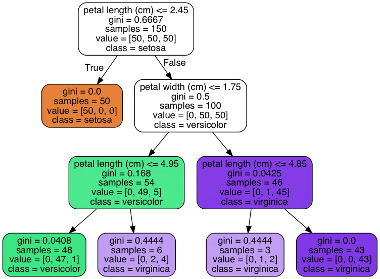
Decision Tree Regression
Decision tree regression is a non-parametric supervised learning algorithm that builds a tree-like model to make predictions. It partitions the feature space into segments and assigns a constant value to each region. For a more detailed introduction and examples, you can click here: decision tree introduction.

Applying decision tree regression using sklearn
Sklearn provides an implementation of decision tree regression through the DecisionTreeRegressor class. It allows customization of parameters such as maximum tree depth, minimum sample split, and the choice of splitting criterion.
Evaluation of decision tree regression models involves using metrics like MSE, R score, and RMSE. Additionally, visualizing the decision tree structure and analyzing feature importance can provide insights into the model’s behavior.
Random Forest Regression
Random forest regression is an ensemble learning method that combines multiple decision trees to make predictions. It reduces overfitting and improves prediction accuracy by aggregating the predictions of individual trees.
Random forest regression offers robustness, handles high-dimensional data, and provides feature importance analysis. However, it can be computationally expensive and less interpretable compared to single decision trees.
Implementing random forest regression with sklearn
Sklearn provides an easy way to implement random forest regression. Here’s an example:
from sklearn.ensemble import RandomForestRegressor
# Create an instance of the Random Forest regression model
model = RandomForestRegressor(n_estimators=100)
# Fit the model to the training data
model.fit(X_train, y_train)
# Predict the target variable for new data
y_pred = model.predict(X_test)
In the code snippet above, X_train represents the training data with independent variables, y_train represents the corresponding target variable values, and X_test is the new data for which we want to predict the target variable (y_pred). The n_estimators parameter specifies the number of trees in the random forest.
Evaluating random forest regression models
Evaluation of random forest regression models involves using metrics like MSE, R score, and RMSE. Additionally, analyzing feature importance and comparing with other regression models can provide insights into the model’s performance and robustness.
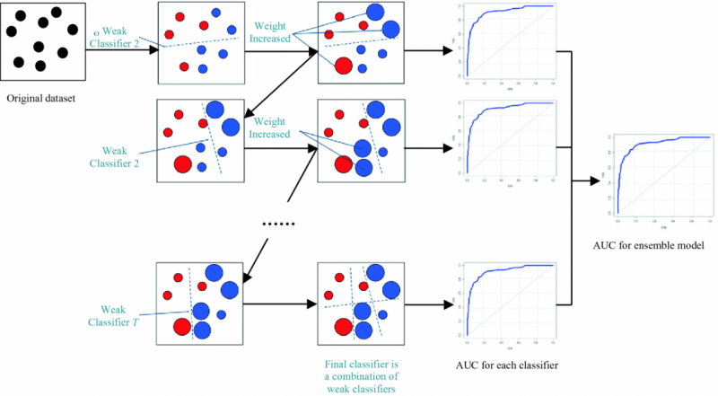
Gradient Boosting Regression
Gradient boosting regression is an ensemble learning technique that combines multiple weak prediction models, typically decision trees, to create a strong predictive model. It iteratively improves predictions by minimizing the errors of previous iterations.
Gradient boosting regression offers high predictive accuracy, handles different types of data, and captures complex interactions. However, it can be computationally intensive and prone to overfitting if not properly tuned.

Utilizing gradient boosting regression in sklearn
Sklearn provides an implementation of gradient boosting regression through the GradientBoostingRegressor class. It allows customization of parameters such as the number of boosting stages, learning rate, and maximum tree depth.
Evaluating gradient boosting regression models
Evaluation of gradient boosting regression models involves using metrics like MSE, R score, and RMSE. Additionally, analyzing feature importance and tuning hyperparameters can optimize model performance. For a more detailed introduction and examples, you can click here: gradient boosting decision trees in Python.
Conclusion
In conclusion, we explored various regression models and discussed the importance of choosing the appropriate model for accurate predictions. Sklearn’s regression models offer a powerful and flexible toolkit for predictive analysis, enabling data scientists to make informed decisions based on data.
The post Mastering Regression Analysis with Sklearn: Unleashing the Power of Sklearn Regression Models appeared first on Datafloq.

